Overview

The steps of this project are follows:

• Compute the camera calibration matrix and distortion coefficients with a set of chessboard images.
• Apply a distortion correction to raw images.
• Use color transforms, gradients, etc., to create a thresholded binary image.
• Apply a perspective transform to rectify binary image (“birds-eye view”).
• Detect lane pixels and fit to find the lane boundary.
• Determine the curvature of the lane and vehicle position with respect to center.
• Warp the detected lane boundaries back onto the original image.
• Output visual display of the lane boundaries and nuemerical estimation of lane curvature and vehicle position.

Tech Stack

• Python
• NumPy
• Scipy
• OpenCV

Camera calibration using chessboard images

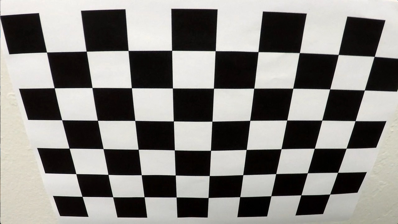
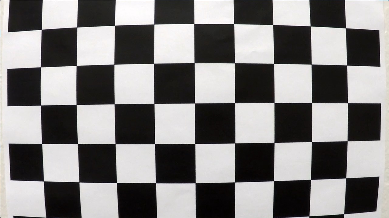
A set of chessboard images photographed at different angles were used for this purpose.

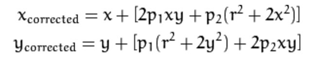
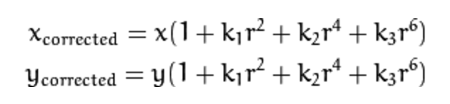
There are two types of distortion in this set of calibration images.

Tangential	Radial

So for each image path:

• image is converted to grayscale using cv2.cvtColor()
• chessboard corners are found using cv2.findChessboardCorners()

Once the chessboard corners are found, cv2.calibrateCamera() is called to obtain the calibration value that will be used to undistort our video images.

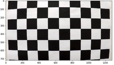
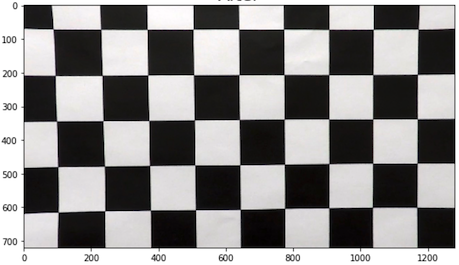
Distortion correction

Using cv2.undistort, the chessboard images can be undistorted.

Original	Corrected

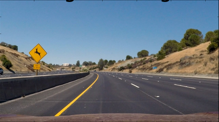
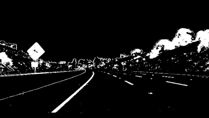
Thresholded binary image

Filters used:

• Gradient on x and y axis with sobel filter size of 5
• HSV for yellow lane lines
• RGB for white lane lines
• S channel with a mask to suppress shadow

These thresholds are combined using logical OR.

Original	Thresholded

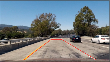
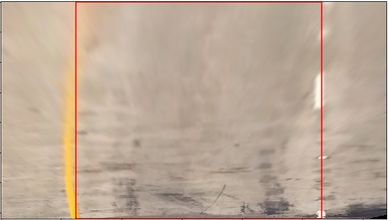
Perspective transform

From an image frame, coordinates are selected in the shape of a trapezoid. The destination coordinates, in the shape of a rectangle, are selected. Using cv2.getPerspectiveTransform, perspective transform M and inverse perspective transform Minv are calculated, which then will be used for image transformation.

def transform_image(img,size,src,dst):
    M = cv2.getPerspectiveTransform(src,dst)
    Minv = cv2.getPerspectiveTransform(dst,src)
    warped_image = cv2.warpPerspective(img,M,size,flags=cv2.INTER_LINEAR)
    return warped_image, M, Minv

Original	Transformed

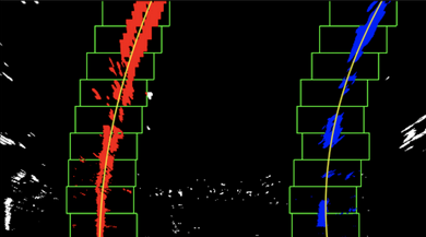
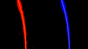
Finding lane lines

Using scipy.signal’s find_peaks_cwt() lane line pixels are calculated. Then using sliding window search, found peaks are then connected to form lines.

Sliding Window Search	Peaks Connected

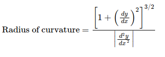
Finding curvature and vehicle position

The curvature of 2nd order polnomial can be calculated with:

def curvature_radius (leftx, rightx, img_shape, xm_per_pix=3.7/800, ym_per_pix = 25/720):
    ploty = np.linspace(0, img_shape[0] - 1, img_shape[0])
    
    leftx = leftx[::-1]  # Reverse to match top-to-bottom in y
    rightx = rightx[::-1]  # Reverse to match top-to-bottom in y
    
    # Fit a second order polynomial to pixel positions in each lane line
    left_fit = np.polyfit(ploty, leftx, 2)
    left_fitx = left_fit[0]*ploty**2 + left_fit[1]*ploty + left_fit[2]
    right_fit = np.polyfit(ploty, rightx, 2)
    right_fitx = right_fit[0]*ploty**2 + right_fit[1]*ploty + right_fit[2]

    # Define conversions in x and y from pixels space to meters
    ym_per_pix = 25/720 # meters per pixel in y dimension
    xm_per_pix = 3.7/800 # meters per pixel in x dimension

    # Fit new polynomials to x,y in real space
    y_eval = np.max(ploty)
    left_fit_cr = np.polyfit(ploty*ym_per_pix, leftx*xm_per_pix, 2)
    right_fit_cr = np.polyfit(ploty*ym_per_pix, rightx*xm_per_pix, 2)
    
    # Calculate the new radii of curvature
    left_curverad = ((1 + (2*left_fit_cr[0]*y_eval*ym_per_pix + left_fit_cr[1])**2)**1.5) / np.absolute(2*left_fit_cr[0])
    right_curverad = ((1 + (2*right_fit_cr[0]*y_eval*ym_per_pix + right_fit_cr[1])**2)**1.5) / np.absolute(2*right_fit_cr[0])
    
    # Curvature and radius in meters
    return (left_curverad, right_curverad)

With the average of the two polynomials (bottom portion), mid point is calculated to determine the vehicle’s position since the camera is assumed to be attached in the middle of the vehicle.

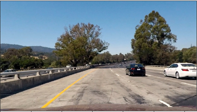
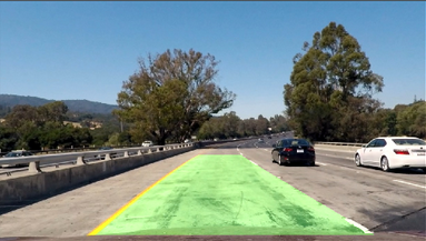
Warp onto the original image

To draw the boundaries onto the original image:

1. Curves are drawn on a blank image.
2. Lane area is drawn by invoking cv2.fillPoly().
3. Using the inverse perspective matrix Minv, the lane area will be warped onto the original image space.

Original	Lane Area Drawn

Completed pipeline